Index | Overview | Regional Syntheses | Global Syntheses | Protocol | Products | Implementation | Sponsorship

REgional Carbon Cycle Assessment and Processes (RECCAP)

Soft Protocol
Version 4

1. Motivation

Available observations are localized and widely separated in both space and time, so we depend heavily on models to characterize, understand, and predict carbon fluxes at regional or global scales. The results from models differ from each other because they use different approaches (forward vs. inverse), modeling strategies (detailed process, statistical, observation based), process representation, boundary conditions, initial conditions, and driver data. We need an approach to identifying the causes of differences and deciding on which formulations and approaches best align with measurements, and why they may or may not agree with measurements.

2. Atmospheric Inversions

Atmospheric inversions or top-down analyses provide estimates of carbon fluxes that are optimally consistent with atmospheric CO2 concentration measurements, but that depend on the choice of an atmospheric transport model. The inversion approach provides coarse scale CO2 fluxes. Its resolution and precision depends on the regional density of atmospheric networks, and on the assigned prior error budgets. Inversions result are ‘comprehensive’ in the sense that all CO2 fluxes, inclusive of fossil fuel emissions, plus all ecosystems sources and sinks plus all other processes emitting or absorbing CO2, are in principle captured by the atmospheric signals. For inversions, it is recommended for the Chapters teams to report in each region of interest:

• Basic data: The net CO2 fluxes on a monthly basis, over the period 1990-2008 - or any approaching period.
• Additional data: Using an ensemble of different inversions is strongly encouraged to assess regional CO2 fluxes and the uncertainties derived from model differences. In that case, how the mean or median of the ensemble is obtained, and how the uncertainty is obtained should be reported. If there is any objective reason for rejecting a model from the ensemble, it should also be explained why.
• Metadata:
  • The area of the region considered
  • For each inversion, what are the characteristics of the method used and relevant references,  and how are the errors calculated

3. Lateral transport

For comparing CO2 fluxes provided by inversions with bottom up estimates from land based C accounting methods and inventories, regionally variable corrections must be made for processes which exchange CO2 with the atmosphere but do not store C in ecosystems. Example of these processes are the use of imported wood and food products releasing CO2, the weathering and river transport of CO2, the CO2 fixed by photosynthesis but leading to the release non-CO2 compounds.

If they can be estimated with regional data, the CO2 fluxes associated with lateral transport should be reported in each region as they help to reconcile and compare bottom up C accounting and top-down inversions. A default regional CO2 flux estimate from crop products trade (Ciais et al. 2007) can be provided. What about for rivers? and for wood products trade? In each region, the method used to estimate CO2 fluxes associated with lateral transport should be reported, and if possible its uncertainties.

4. Forward, large scale or bottom-up terrestrial ecosystem models

Ecosystem models can be used to test hypotheses concerning the attribution of processes in determining carbon fluxes and make projections using forcing scenarios. Examining and comparing results of inverse and forward model simulations with each other and with suitable measurements can help evaluate model strengths and weaknesses, and utility, and provide multiple views of regional patterns of fluxes, lead to understanding of processes involved, and provide a basis for making projections.

The forward or bottom-up models can provide analysis results at the temporal and spatial resolution of simulation runs more-or-less in hand. These will range from hourly to annual time steps. For bottom up models, it is recommended for the Chapters teams to report in each region of interest:

• The net ecosystem exchange CO2 fluxes on a monthly basis, at the model original spatial resolution over the period 1990-2008 - or any approaching period,
• The area of the region considered,
• The components of net ecosystem exchange including GPP, NPP, Ra, Rh, Fire and other disturbances, on a monthly basis,
• Other diagnostic components that can be compared to global observations in particular LAI, above ground biomass, evapotranspiration, soil moisture, and soil carbon on a monthly basis,
• Using different ecosystem models is strongly encouraged to assess regional CO2 fluxes and the uncertainties derived from model differences. The underlying model parameterizations and assumptions should be described in a summary table. The sources of input data for land cover, climate and CO2, possibly for Nitrogen deposition should be referenced. For data oriented models, or data fusion products the source of input data should be given.

5. Large scale biomass and soil carbon inventory data

Inventory data are maybe the most precious source of observation to quantify long-term and regional patterns in the carbon balance of continents. But they are limited to extra-tropical regions. These data can be used to evaluate models and if repeated inventory surveys are available, to quantify cumulated changes in C over time. For RECAPP, we recommend inventory results to be reported in C mass and C flux units at the best possible spatial coverage (e.g. small administrative units, or even on a regional grid). Land cover maps associated with the provision of data on C stock changes will be needed. Description of the allometry methods used to convert tree diameter increment into volume and whole tree biomass should be given. If a model used to estimate soil C changes from forest inventory data, this model should be described in the same way as the ecosystem models above.

6. Ocean CO2 observations products

Two approaches have been used to understand ocean carbon uptake and storage. One approach is to assess ocean carbon inventory changes in the ocean interior. This is accomplished by reoccupying ocean sections that were surveyed during the 1990s. This work provides information on the decadal scale changes in ocean carbon storage. The second approach is to estimate air-sea CO2 fluxes. Surface ocean and atmospheric CO2 partial pressure is measured from ships of opportunity and moorings. These data are used to develop empirical relationships with properties that can be observed from satellites. Using the time and space coverage of the satellite observations we can generate global fluxes at monthly to decadal time scales. Both the surface observations and the ocean interior observations are used to better understand the controls on the ocean’s role in the global carbon cycle.

Air-sea flux estimates:

• Basic data: sea-air CO2 flux at monthly over the original grid of estimate, for 1990-2008. Units of mol m-2 y-1.
• Additional data: grid, pCO2, SST, wind speed, data statistics (number of data per grid point, variance etc), atmospheric pCO2.
• Metadata: pCO2 measurement technique, gas exchange model, method to interpolate data.

Ocean interior carbon changes:

• Basic data: Decadal changes in dissolved inorganic carbon along ship cruise tracks in all oceans.
• Additional data:
• Metadata:

7. Ocean models

Ocean models can be used to test the impact of climate change on the air-sea CO2 fluxes, and to project the oceanic CO2 sink into the future. The reliability of the models can be determined by the examination of the CO2 fluxes over the historical period and their comparison with atmospheric and oceanic inversions and in situ data.

• Basic data: sea-air CO2 flux at monthly resolution on a regular grid for (a) 1990-2008 averaged, and (b) each month during 1959-2010 or subset based on availability. Units of mol m-2 yr-1.
• Additional data: grid, pCO2, SST, SSS, DIC (sfc), Alk (sfc), mixed layer depth, biological export at 100 m, NPP. 
• Metadata: model description (physics, bgc, ecology), surface forcing, spin-up, gas exchange model, key parameterizations, river fluxes (if considered)

Additional option: (a) results from simulations that separate "natural" from "anthropogenic" CO2, (b) simulations with variable and constant forcing.

8. Oceanic Inversions

Oceanic inversions provide estimates of CO2 fluxes based on the distribution of passive tracers in the ocean. It is essentially an observation-based estimate, although oceanic transport from models is used to relate observed concentrations to fluxes. This method gives CO2 fluxes directly, and thus it is not limited by the large uncertainty in gas exchange. The currently applied method provides estimates of the long-term mean annual flux.

• Basic data: Long-term mean annual sea-air CO2 flux for a nominal year of 1995 and 2000. Units of mol m-2 yr-1.
• Additional data: grid, areas of grid cells, region boundaries, within region flux pattern, prior and posterior uncertainties (within and between models if multiple transport models were used) 
• Metadata: inversion methodology, data used, regularization constraints (if used), model description.

Additional option: “natural” versus “anthropogenic” fluxes.

9. C4MIP models

Suggestion: should we also have the runs by the chosen regions and basins from the C4MIP?

10. Regional RECAPP Server

We will create a central data repository that will house data, model descriptions,
documentation, and analysis results. GCP will provide some standard software tools and assistance to help participants convert data and model output into the standard format for use in model-data comparison. We will incorporate standard security procedures to ensure only MIP participants can access the repository. In addition, we will implement a data fair use policy.

11. Data and Model Output Fair Use policy

The project will involve scientists from a large number of independently funded research projects. To ensure the individuals and teams that provide model output and data receive proper credit for their work, we have instituted a Fair Use Policy. The policy applies to all data and model output stored on the Regional MDC server. The Fair Use Policy is based on the Ameriflux Policy, but expanded to include all Site MDC participants:
The data and model output provided on this site are freely available and were furnished by individual scientists who encourage their use. Please kindly inform in writing (or email) the appropriate participating scientist(s) of how you are using the data and of any publication plans. If not yet published, please reference the source of the data or model output as a citation or in the acknowledgments. The scientists who provided the data or model output will tell you if they feel they should be acknowledged or offered participation as authors. We assume that an agreement on such matters will be reached before publishing and/or use of the data for publication. If your work directly competes with an ongoing investigation, the scientists who provided the data or model output may ask that they have the opportunity to submit a manuscript before you submit one that uses their data or model output. When publishing, please acknowledge the agency that supported the research. We kindly request that those publishing papers using AmeriFlux data, Fluxnet Canada data, or Regional MDC model output provide reprints to the appropriate scientist providing the data or model output, and to the data archive at the Carbon Dioxide Information Analysis Center (CDIAC).

12. Regional Email Lists

The RECAPP synthesis involves a large number of modelers, experimenters, observationalists, program managers. To facilitate effective communication, we will create participant email lists to disseminate information. As required, we will create smaller email lists consisting of subsets of the full participant list to focus on specific problems or research efforts

13. Information Provided by Participants

All potential model participants should provide general descriptive information
about the model they used to produce their results. This includes a short model overview (1-2 paragraphs) with a brief description, basic structure, model initialization procedure, description of driver data, web pages, and associated references. Participants should also provide a primary point of contact and, if desired, secondary points of contact for each model. Lastly, we recognize that the required inputs for each model differ, so the participants should provide a list of all inputs used by their model. In particular, vegetation type or land cover classification should be provided. This will allow some subsetting of results for comparisons by vegetation types.
Data providers should provide a short overview of their measurements, a description of how they are derived, estimates of uncertainty, and associated references.

14. Inputs to Model

We will not prescribe model driver data. Weather, phenology, soil properties, N deposition, etc. is left up to the modeling teams. For addressing the question of the absolute size of the carbon sources and sinks, initialization of carbon pools will be important and each participant should provide a description of their initialization technique. Those models with nitrogen or phosphorus biogeochemistry should initialize those variables as best suited for their model and provide a description of the procedure.

The best file format for providing spatial model output is CF compliant netCDF.
An example will be provided on the MAST-DC ftp site. Instructions for producing such a file from ASCII files and appropriate meta-data will be developed if necessary. These instructions provide additional guidance on what information will be required for model output. Software tools for most computer platforms for producing and viewing netCDF files is available. See http://www.unidata.ucar.edu/software/netcdf/ for general information and http://cf-pcmdi.llnl.gov/ for a complete description the CF convention for netCDF files. As a concrete example, please see
ftp://ftp.cmdl.noaa.gov/ccg/co2/carbontracker/regions.nc. This CF-1.0 and COARDS compliant netCDF file not only defines the grid but also gives Transcom 22 region definitions on that grid. We will also accept netCDF files with the ALMA convention (see http://web.lmd.jussieu.fr/~polcher/ALMA/dataex_main.html). If a data or modelling team has difficulty in translating files to netCDF contact us and we’ll do what we can with limited MAST-DC resources to help. Do not assume that if your files are not in netCDF format that you are eliminated from participating.

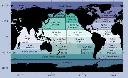
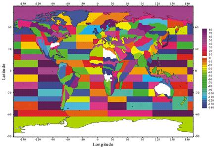
15. RECCAP regions

RECCAP needs to define the regions of interest in order to interrogate data and model in a consistent way and to prepare key datafiles for distribution to all participants. Given that global models run on a grid basis they can be aggregated on any region of interest.

The regions shouldn’t be too coarse to avoid masking interesting results, or hinder in-depth analysis. They shouldn’t be too fine either given the limited data defining that region (eg, inversions).

The map below is an initial proposal with a compromise for inversions between pixel-based inversion and the very coarse TransCom regions which lack biogeochemical meaning. The region contours are drawn from land cover (over land) + expert judgement on where the atmospheric stations actually exist, to avoid some aggregation errors (eg you don't want one station in Japan to constrain a steppe flux over a long strip going from Ukraine to the Far east in longitude). For the ocean, the number of regions should be reduced to no more than the number of regions used for the recent ocean inversions (23)../../..

RECCAP Ocean Regions_MAP1

RECCAP Ocean Regions_MAP2

16. Regional Synthesis: Methods Land Regions

We acknowledge the fact that coverage of each region by inventories, atmospheric networks and flux towers is quite uneven. To ensure that global coverage will be available, while leaving open the possibility for regionally more detailed or higher resolution estimates, the data will be divided into two tiers.

Tier 1

Gridded output of from at least three process-based terrestrial biosphere models ORCHIDEE, JULES, LPJ. These runs will be performed under the QUEST benchmark. Additional data-driven model estimates (e.g. based upon Remote sensing, eddy flux data) will also be provided.

Datasets

Gridded output of GPP, NPP, Rh, NBP, main C stocks (netcdf file) ; Spatial resolution = 0.5° ; temporal resolution =f 1 month ; (maximum) period 1981-2008. Flux units gC m-2  month-1. Stock Units KgC m-2

Mean values of these variables in a separate text file.

RECAPP core group will provide these data to all participants

Tier 2

Detailed regional flux and pools estimates from various regional data sources and sectorial models. Gridded files over the same regions than defined for Tier 1 are expected, including for data originally collected on a non-regular grid ;

Datasets
Gridded out put of GPP, NPP, Rh, NBP, main C stocks and other relevant fluxes (e.g. lateral, wood products, freshwaters) Flux units gC m-2 month-1. Stock Units KgC m-2

Recommended spatial resolution of ≈10 km ; temporal resolution monthly. If higher resolution datasets are available, provide std. dev. within each 10 km grid cell.

Target period is 1981-2008. If a shorter measurement period is covered or if monthly resolution is impractical (e.g. for biomass inventories) then length of measurement period and temporal resolution should be reported separately.

Mean values of these variables in a separate text file.

Each Regional Chapter lead will provide Tier 2 data

RECAPP core group will distribute these data to all participants